2.2. Using the ACT

To use the ACT, you first need to install the ACT. Once you have finished that, please try the command:

alexandria -h

and:

alexandria help commands

the output of which is given in Table 2.2 .

Table 2.2 Commands available in the alexandria program.

Command	Description
analyze	Analyze molecular or force field properties from a database and generate publication quality tables in LaTeX.
b2	Compute second virial coefficient as a function of temperature.
edit_ff	Manipulate and compare force field files in various ways and test whether reading and writing works.
edit_mp	Utility to merge a number of molecular property files and a SQLite database. Can also test reading and writing the molecular property file. It can also check the molecular property file for missing hydrogens and for whether it is possible to generate topologies for all compounds. Finally it can generate charges for all compounds.
gen_ff	Generate a force field file from a user specification.
gentop	Generate a molecular topology and coordinates based on structure files. Only inputs for OpenMM can be generated at this point in time.
geometry_ff	Deduce bond/angle/dihedral distributions from a set of structures and add those to a force field file.
help	Print help information.
merge_ff	Utility to merge a number of force field files and write a new file with average parameters. Can also write a LaTeX table.
min_complex	Generate inputs for an energy scan.
nma	Perform normal mode analysis and compute vibrational frequencies and thermochemistry properties.
simulate	Perform a MD simulation and generate a trajectory.
train_ff	Train a force field to reproduce reference data.

Note that one can get detailed help for the alexandria modules using the -h flag, e.g.:

alexandria train_ff -h.

In addition to the alexandria program, the ACT contains a number of python scripts and utilities (Table 2.3 ), some of which are needed for the quantum chemistry calculations as well (see Sections Generating SAPT data and Generating single molecule data).

Table 2.3 Python utilities available in the ACT.

Command	Description
coords2molprop	Read a bunch of structure files containing molecule dimers A-B and write a molprop file.
dimer_scan	Compute dimer potentials for along a user-defined distance between two molecules.
donchev2molprop	Convert dimer interactions from the Donchev paper [28] to a molprop file.
gauss2molprop	Read a Gaussian output file from the Alexandria library [17] to a molprop file.
generate_mp	Read and process many Gaussian output files from the Alexandria library [17] and generate a molprop file.
install_act	Script to install the ACT
molselect	Make a selection file based on compounds from the Alexandria Library.
ncia2molprop	Read an xyz file and write a molprop file.
plot_convergence	Read an ACT training log file and plot the converge of the parameters as a function of generations in the evolution of the gene pool.
reshuffle_selection	Read a selection file and randomly assign Train status to entries, then write a new selection file.
view_fitness	Visualizes the fitness per generation of a GA/HYBRID by plotting the maximum, minimum, mean, and median, for an example see Fig. 2.1

Fig. 2.1 Sample convergence plot from a HYBRID training, generated by the view_fitness script.

2.2.1. ACT File formats

The ACT contains a number of specific file formats, in principle all of them generated by the ACT itself through scripts (Table 2.3) or alexandria (Table 2.2). The files are listed below:

• Selection file, with .dat extension. List of monomers or dimers and designation on whether they are part of the train or test set. In case of dimers, the two compounds are separated by a hash (#) symbol.:

  water#ethanol|Test
  water#water|Train
  ethanol#ethanol|Train
  

• Force field file, with .xml extension.

• Molprop file, with .xml extension.

2.2.2. Creating a new force field file from scratch

Start by copying the examples directory from the source catalog, and change directory to examples/NonPol.

Now, let’s see what alexandria gen_ff has to offer:

alexandria gen_ff -h

(to see the output check the help text).

As we see there are many options, but for Alexandria force fields most can remain default. Make a fresh directory and use the one-line script:

./genff.sh

which gives output similar to:

There are 62 atom types in the force field with 42 properties.
There are 127 element properties

Thanks for using the Alexandria Chemistry Toolkit.

The script prints that it has read and processes a number of files from the ACT installation. These data files can be copied and modified by the user. The files should be relatively simple to understand. Installed files are in the share/act directory. Please note that the force field files use the eXtensible Markup Language that provides a structured way of storing data. Do not edit manually if at all possible.

This force field file gives us something to start with, but it is not complete yet. First, we have to add the possible bond lengths, bond angles etc., and those come from the Alexandria Library (see below). For now, we will use the provided file in XML/alcohol.xml. Thus, we need to run:

./geomff.sh

which should produce the following output:

   Welcome to the Alexandria Chemistry Toolkit

There are 5 molecules in the selection file SELECTIONS/alcohol-monomer.dat.
There are 5 molprops. Will now sort them.
There were 0 double entries, leaving 5 after merging.
There were 5 total molecules before merging, 5 after.
Have generated 34 entries for bond charge correction (SQE algorithm).

Please check output in file geometry_ff.log.

This generates a ready-to-optimize force field file, myff2.xml and a log file that is good to inspect. It provides statistics over the geometry of compounds in the input xml file:

bond-c3_b~h_b len 108.8 sigma 0.3 (pm) N = 28
bond-c3_b~c3_b len 150.9 sigma 0.6 (pm) N = 7

angle-c3_b~c3_b~c3_b angle 112.1 sigma 0.6 (deg) N = 3
angle-c3_b~c3_b~o3_b angle 108.6 sigma 3.8 (deg) N = 7

which informs us, for instance, that there are 28 aliphatic c3-h bonds in the input with an average length of 108.8 \(\pm\) 0.3 pm.

2.2.3. Train your first force field

Now you can run the first part of the example training, the intermolecular interactions, using:

./run_inter.sh

and the adventure has begun! This part will train the van der Waals parameters \(\sigma\) and \(\epsilon\) (Eqn. (3.18)) as well as the charge distribution width \(\zeta\) (Eqn. (3.2)) and the electronegativity \(\chi\) and hardness \(\eta\). The command will output some text to the terminal:

There are 16 threads/processes and 5 parameter types to optimize.
rank: 0/16 nodetype: Master superior: 0
nmiddlemen: 16 nhelper_per_middleman: 0
ordinal: 0 nhelper: 0
middlemen:   1   2   3   4   5   6   7   8   9  10  11  12  13  14  15

showing the genetic algorithm is using 16 individuals and the code is being run on 16 threads in parallel. Then, at the end you will see something like:

There were 39 EPOT-Train outliers for Train.
There were 29 EPOT-Test outliers for Test.

Please check output in file train_inter.log.

encouraging you to inspect the log file. It can be very helpful to check outliers that can help you to find inconsistencies in both the data and the model you are trying to train. After this training instance, a correlation plot EPOT.xvg will be produced (Fig. 2.2); you can use the:

./plot-epot.sh

script to make the plot yourself as well.

Fig. 2.2 Correlation between interaction energy from SAPT (x-axis) and training (y-axis).

You can inspect the different .xvg output files in the generated subdirectory inds. Fig. 2.3 shows how the total deviation from SAPT data, you can recreate the figure using the:

./plot-chi2.sh

script. Fig. 2.4 shows how well the Gaussian distribution widths converge.

Fig. 2.3 Convergence of the \(\chi^2\) fitness value for the first individual in the example training. Note the jump at iteration 100, due to the catastrophe penalizer kicking in.

Fig. 2.4 Convergence of the Gaussian distribution widths \(\zeta\) for five atom types. The jumps in the graphs are due to genetic algorithm performing crossover between individuals.

Note that these graphs were made using the plotxvg script that is based on matplotlib.

After training the parameters governing intermolecular interactions, it is time to train the bonded forces. For this, we need to modify the selection of compounds to be monomers, we use the force field file that was trained on SAPT interaction energies (Train-inter.xml) and reference energies come from MP2 calculations.

./run_intra.sh

will do this training. As targets in this training we use both the intramolecular energies and the forces, however the deviations in the forces are weighted down by a factor of 0.1 because of the magnitude of the numbers. You will get similar output as for the intermolecular training:

There were 60 EPOT-Train outliers for Train.

Please check output in file train_intra.log.

Again, please inspect the contents of the log file carefully. A quick check of the intramolecular force field can be done by computing frequencies:

./run_nma.sh

which will perform a normal mode analysis (Sec. Normal Mode Analysis) and compute an infrared spectrum (Sec. Infrared Spectra) based on your new force field. This should yield a spectrum like the one in Fig. 2.5.

Fig. 2.5 Simulated infrared vibrational spectrum for ethanol based on the force field derived in this tutorial (please compare to Fig. 2.7).

As a final test of your new force field, we can use alexandria simulate -minimize to determine the optimized structure of a methanol dimer. For this, run:

./minimize.sh

and check the output structure, after_em.pdb. It should look like Fig. 2.6.

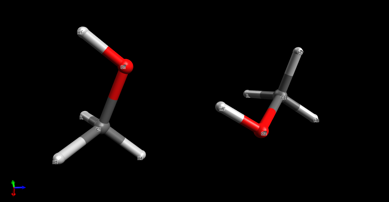
Fig. 2.6 Structure of a methanol dimer after minimization using the force field derived by the ACT in this tutorial. Visualization using Avogadro.

Please make sure to inspect all the scripts provided here to learn about the command line options to ACT modules, but be advised that there are many more options and possibilities.

To design a force field for your own system of choice you will have to provide quantum chemistry data (Sec. Training Data), and create selection files (Sec. ACT File formats). Most of the steps you have gone through in this tutorial can be adapted to your need. For large trainings it is useful to study the parallellization features of the ACT (Sec. Running training using parallel processing).

2.2.4. Is my training hitting a wall?

To make training efficient, it is good to limit the search space. In some cases we can use chemical intuition to estimate the search space. For instance, we know that polarizability should be a positive number and that it is highly element dependent. For hydrogen, a likely range is 0.1 < \(\alpha <\) 0.5 \(\text{\AA}^3\). Such boundaries are implemented in the force field file like this:

<parameterlist identifier="h_s">
  <parameter type="alpha" unit="Angstrom3" value="0.46"
  uncertainty="0.008" minimum="0.1" maximum="0.5"
  ntrain="300" mutability="Bounded" nonnegative="yes"/>
</parameterlist>

this example is after an optimization where the optimal value ended up being 0.46, based on a dataset comprising 300 hydrogen atoms. Note the nonnegative=”yes” which will prevent alexandria tools from making this parameter negative ever.

For many cases, we do not have an {em a-priori} intuition of what the values should be and we make a guess. Then, after a series of optimizations, we can check whether the bounds are OK, using an alexandria tool (assuming you have generated and trained a polarizable force field .xml ):

alexandria edit_ff -ff ff.xml -ana EEM
<snip>
POLARIZATION n2_s alpha at maximum 1.5
POLARIZATION n4_s alpha at minimum 0.6
BONDCORRECTIONS c2_~c3_z hardness at minimum -0.4
BONDCORRECTIONS c2_z:n2_z hardness at minimum 0
BONDCORRECTIONS c3_z~c3_z hardness at minimum -0.4

Some of the parameters are indeed hitting the wall. To adjust the parameters we use the same tool again:

alexandria edit_ff -ff ff.xml -o new.xml -stretch -p alpha
<snip>
Thanks for using the Alexandria Chemistry Toolkit.

and then we check the resulting force field file in the same manner as before:

alexandria edit_ff -ff new.xml -ana EEM
<snip>
BONDCORRECTIONS c2_z~c3_z hardness at minimum -0.4
BONDCORRECTIONS c2_z:n2_z hardness at minimum 0
BONDCORRECTIONS c3_z~c3_z hardness at minimum -0.4

Now the polarizability minimum (for n4_s) and maximum (for n2_s) have been stretched. The same can now be done for hardness.

You can also do the reverse. When you are confident that the optimization is close to the final result, but want to randomize again without starting from scratch, you can set new minimum and maximum values for the parameters using, e.g.:

alexandria edit_ff -ff new.xml -o new.xml -p bondlength -limits 0.98

please check the on-line help ( alexandria edit_ff -h ) for more information.

2.2.5. Running training using parallel processing

The training process is heavy in computer time. Therefore, it has been parallellized using the MPI library. Since this is a prerequisite for compiling the ACT, you likely have it installed if you got this far. In fact this is used in the example scripts, where N is the number of cores you have available. Please consult with your cluster manager if in doubt. Clusters using the Slurm queueing system may need to use srun instead of mpirun. As far as we have tested [1], the code is quite efficient down to 4-5 molecules per core. In the above example there are 10 compounds in the training set, such that it is not worthwhile to use more than 2-3 cores, but do experiment with the number of cores.