3.2. Force Field Training Algorithms¶

This chapter was written by Juli{'a}n Marrades and is based in part on his M.Sc. thesis :cite:p:`Marrades2022a`.

Within the alexandria train_ff module of the Alexandria Chemistry Toolkit you can choose among three algorithms to optimize force field parameters:

Markov Chain Monte Carlo (flag -optimizer MCMC)
Genetic Algorithm (flag -optimizer GA)
Hybrid GA/MCMC (flag -optimizer HYBRID)

Let us see what they do behind the scenes and how to control them.

3.2.1. MCMC¶

Assume we want to set the values for five parameters (nParam = 5) by performing ten MCMC iterations (flag -maxiter 10). Then, the code “reads”

for (int i = 0; i < 10; i++)
  for (int j = 0; j < 5; j++)
    stepMCMC();

That is, we do 10 X 5 = 50 MCMC steps. What is a MCMC step though? In essence,

prevDev: previous deviation from data
Choose a parameter and alter it
newDev: new deviation from data
If newDev < prevDev, we accept the parameter change and continue into the next step. Else, apply Metropolis Criterion. That is, with some probability we accept the change. Otherwise, we restore the parameter to its previous value and proceed into the next step.

Now, let us add some more detail to the algorithm.

we already have the deviation from data of the previous step in prevDev.
we arbitrarily choose a parameter out of the param vector, say param[i], which is bounded by its maximum pmax[i] and its minimum pmin[i], yielding the range prange[i] = pmax[i] - pmin[i]. Here is where the -step [0, 1] flag comes into play by specifying a fraction.\
we draw a value of delta, which is uniformly distributed in [- step * prange[i], + step * prange[i]] and add it to the parameter value param[i] += delta. If the parameter has gone beyond its maximum, we set its value to the maximum. Same goes for the minimum.<br>
we compute the deviation newDev from data of the modified parameter vector. If newDev < prevDev, we accept the change and finish the MCMC step. Otherwise, we apply the Metropolis Criterion and finish the step. Then go back to 1.

3.2.1.1. Metropolis Criterion¶

If Mathematics is your thing and you {em really} want to know the nitty-gritty stuff, you have thorough explanations of this method on href{https://en.wikipedia.org/wiki/Metropolis%E2%80%93Hastings_algorithm}{Wikipedia} and Shuyi Qin’s Master thesis [91]. Here, we shall say that the Metropolis Criterion allows us to take steps that do not get us closer to a minimum, giving the opportunity to explore the parameter space and avoid local minima. How exactly?

The probability of accepting a “bad” parameter change is controlled by the flag -temp T flag and follows the equation

\[prob = exp(-deltaDev/T)\]

where deltaDev = newDev - prevDev. Note that the unit of temperature is the same as that of the deviation.

Given deltaDev, a higher temperature gives a higher probability of acceptance, as -deltaDev/T tends to 0 and exp(0) = 1. On the other hand, a lower T gives less chances of acceptance, as -deltaDev/T tends to \(-\infty\) and \(exp(-\infty)\) = 0.

ACT gives us the possibility to lower the temperature (simulated annealing) during the MCMC optimization with the flag -anneal [0, 1] flag. If we use flag -anneal 0.5, the temperature will be flag -temp T until 50% of the iterations have been completed. Then, it will be linearly decreased until it reaches 0 on the last iteration.

There are two remarks to be made here:

The temperature is kept constant during the nParam MCMC steps that take place for a given iteration.
Since division by 0 is not defined, we set T = 1e-6 on the last iteration.

Fig. 3.2 shows a schematic example of the temperature over time when we use actflag{-maxiter 10 -temp 5 -anneal 0.5}.

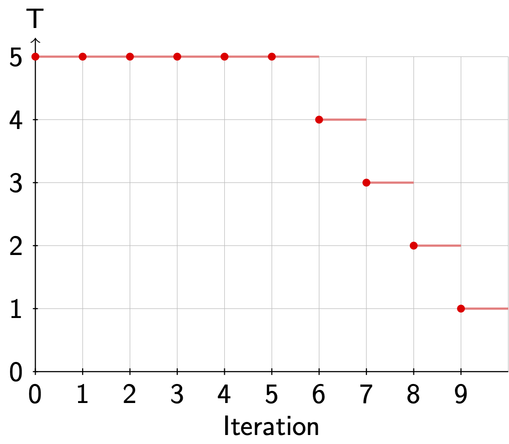
../_images/annealing.png — Fig. 3.2 Annealing during a MCMC run.¶

3.2.1.2. Multiple MCMC runs¶

We can optimize several candidate solutions in parallel using the -pop_size flag. If the -random_init flag is set (default), each candidate solution will be initialized arbitrarily and respecting parameter ranges. If -norandom_init is employed, the candidate solution(s) will be initialized as specified by the force field file(s) provided by the user.

3.2.2. Genetic Algorithm¶

Quoting WikipediaGA

In computer science and operations research, a genetic algorithm is a metaheuristic

inspired by the process of natural selection that belongs to the larger class of

evolutionary algorithms. Genetic algorithms are commonly used to generate

high-quality solutions to optimization and search problems by relying on biologically inspired operators such as mutation, crossover and selection.

In this section, we describe our implementation of a genetic algorithm for force field parameterization. If this is the first time you hear about genetic algorithms and want to acquaint yourself, we recommend you to read Chapter 2 of Steven F. van Dijk’s PhD thesis [92] and/or head over to Youtube.

Our implementation is based upon a class definition and an external function for computing random numbers (Listing Class definition. ).

Listing 3.1 Class definition.¶

class Genome
{
    double params[];
    double deviation;
    double probability;
};

// Returns a sample of a random variable that is
// uniformly distributed in [0, 1]
double random();  

then the genome evolution boils down to the code in Listing Schematic of the evolution algorithm

Listing 3.2 Schematic of the evolution algorithm¶

void evolve(int popSize, int nElites, int prCross, int prMut)
{
    Genome oldPop[popSize] = initialize(popSize); // Initialize
    Genome newPop[];
    computeDeviation(oldPop); // Deviation from data
    int generation = 0;
    do
    {
        sort(oldPop); // Sorting
        if (penalize(oldPop, generation)) // Penalty?
        {
            // Recompute deviation and sort again
            computeDeviation(oldPop);
            sort(oldPop);
        }
        generation++;
        computeProbabilities(oldPop); // Selection probabilities
        // Elitism
        for (int i = 0; i < nElites; i++)
            newPop.add(oldPop[i]);
        // Rest of population
        for (int i = nElites; i < popSize; i += 2)
        {
            Genome parent1, parent2 = select(oldPop); // Selection
            Genome child1, child2;
            if (random() <= prCross) // Crossover?
                child1, child2 = crossover(parent1, parent2);
            else
                child1, child2 = parent1, parent2;
            // Mutation
            for (Genome child : {child1, child2})
            {
                mutate(child, prMut);
                newPop.add(child); // Add to new population
            }
        }
        computeDeviation(newPop); // Deviation from data
        oldPop = newPop; // Swap populations
        newPop.clear();  // Erase all genomes in the population
    }
    // Termination
    while (!terminate(oldPop, generation));
}

flag popSize and flag nElites are assumed to be even. Let us explore the different stages of the process.

3.2.2.1. Initialization¶

This stage fills the params field in the Genome class, generating popSize (flag -pop_size) genomes.

If we are using flag -norandom_init, the genomes will be initialized as specified by the force field file(s) provided. If we are employing flag -random_init, each genome will be initialized by setting a random value for each parameter, uniformly distributed over the allowed range.

3.2.2.2. Deviation from data¶

Here we fill the deviation field in for each Genome in the population by computing the deviation from the dataset.

3.2.2.3. Sorting¶

Sorting is not a mandatory step but may be required depending on the GA components selected by the user. We sort the population in ascending order of deviation. Whether we sort or not is controlled by the flag -sort flag.

3.2.2.4. Penalties¶

At this stage, we may alter the population if certain conditions are met, with the main goal of preventing premature convergence and enforcing solution diversity.

Covering such a small portion of the space you are. Broaden your search, you should. - Yoda

To that end, we have a function penalize() which returns true if the population was penalized and false otherwise.

For now, there are two components in this function:

Volume. This option enables flag -sort. If the volume spanned by the population divided by the total volume of the parameter space is smaller than flag -vfp_vol_frac_limit [0, 1]|, the {em worst} fraction flag -vfp_pop_frac [0, 1] of genomes in the population will be randomly reinitialized. If flag -log_volume is used, volumes will be computed in logarithmic scale. * But wait, then the volume could be negative! Yes, we have to fix that!*

Death comes equally to us all, and makes us all equal when it comes. - John Donne
Catastrophe. Each flag -cp_gen_interval generations, a fraction flag -cp_pop_frac [0, 1] of the genomes in the population will be randomly reinitialized. Genomes to reinitialize are arbitrarily chosen.

3.2.2.5. Selection probabilities¶

We provide three options for computing selection probabilities:

Rank (flag -prob_computer RANK)
Fitness (flag -prob_computer FITNESS)
Boltzmann (flag -prob_computer BOLTZMANN)

The sum of the selection probabilities of the genomes in the population, is 1.

3.2.2.6. Rank¶

This option enables flag -sort. The selection probability depends exclusively on the index (rank) of genome in the population (Listing Calculation of the probability from the order of probabilities.).

Listing 3.3 Calculation of the probability from the order of probabilities.¶

for (int i = 0; i < popSize; i++)
{
  oldPop[i].probability = (popSize - i) / (popSize * (popSize + 1) / 2);
}

That is, the lower the index, the higher the probability of being selected. The independence of the deviation avoids the possible phenomena of a genome with a very high selection probability dominating the population.

3.2.2.7. Fitness¶

The selection probability is inversely proportional to the deviation (Listing Calculation of the probability from the deviations from data.).

Listing 3.4 Calculation of the probability from the deviations from data.¶

double total = 0;
double inverses[popSize];
double epsilon = 1e-4;
for (int i = 0; i < popSize; i++)
    inverses[i] = 1 / (epsilon + oldPop[i].deviation);
    total += inverses[i];
for (int i = 0; i < popSize; i++)
    oldPop[i].probability = inverses[i] / total;

3.2.2.8. Boltzmann¶

The temperature parameter is specified by the flag -boltz_temp flag and controls the smoothing of the selection probabilities (Listing Use of Boltzmann-weighting when calculating the probability). A higher value will avoid polarization in the probability values and vice versa. The flag -boltz_anneal flag allows us to decrease the temperature over time and has the same logic as flag -anneal, except that it targets the Boltzmann selection temperature and operates based on the maximum amount of generations.

Listing 3.5 Use of Boltzmann-weighting when calculating the probability¶

double total = 0;
double exponentials[popSize];
double epsilon = 1e-4;
for (int i = 0; i < popSize; i++)
    exponentials[i] = exp(1 / (epsilon + oldPop[i].deviation) / temperature);
    total += exponentials[i];
for (int i = 0; i < popSize; i++)
    oldPop[i].probability = exponentials[i] / total;

3.2.2.9. Elitism¶

In order to avoid losing the best candidate solutions found so far, the GA will move the top nElites flag -n_elites genomes, {em unchanged}, into the new population. That means, the genome will not undergo crossover nor mutation.

When flag -n_elites > 0, flag -sort will be enabled.

3.2.2.10. Selection¶

Once the selection probabilities are computed, the population becomes a href{https://en.wikipedia.org/wiki/Probability_density_function}{probability density function} from which we can sample genomes based on their probability.

As of now, only a vanilla selector is available. It only looks at the probability and can select the same genome to be parent1 and parent2.

3.2.2.11. Crossover¶

With certain probability prCross, controlled by the flag -pr_cross flag, two parents will combine their parameters to form two children. Right now, only an N-point crossover is available, where N is defined by the flag -n_crossovers flag.

If N = 1, we arbitrarily select on crossover point (v) and:

    v                        v
|X|X|X|X|X|X|X|X|X|  --> |X|X|Y|Y|Y|Y|Y|Y|Y|
|Y|Y|Y|Y|Y|Y|Y|Y|Y|  --> |Y|Y|X|X|X|X|X|X|X|

If N = 2, we arbitrarily select two crossover points (v) and:

  v     v                  v     v
|X|X|X|X|X|X|X|X|X|  --> |X|Y|Y|Y|X|X|X|X|X|
|Y|Y|Y|Y|Y|Y|Y|Y|Y|  --> |Y|X|X|X|Y|Y|Y|Y|Y|

If N = 3, we arbitrarily select three crossover points (v) and:

       v     v     v            v     v     v
|X|X|X|X|X|X|X|X|X|  --> |X|X|Y|Y|Y|X|X|X|Y|
|Y|Y|Y|Y|Y|Y|Y|Y|Y|  --> |Y|Y|X|X|X|Y|Y|Y|X|

If N = 4… you get the idea (hopefully).

3.2.2.12. Mutation¶

Given the mutation probability prMut, controlled by flag -pr_mut, we iterate through the parameters. If the probability is met, we alter the parameter, otherwise, we leave it unchanged.

for (int i = 0; i < nParams; i++)
{
  if (random() <= prMut)
  {
    changeParam(params, i);
  }
}

The parameter is changed in the same way as in MCMC, by a fraction of its allowed range and not allowing values outside of it. The fraction in this case is controlled by the -percentage flag, which has the same meaning as -step, but applies to GA instead of MCMC.

3.2.2.13. Termination¶

This stage decides whether the GA evolution should continue or halt. We allow the user to tweak the termination criteria with several flags:

flag -max_generations: evolution will halt after so many generations.
flag -max_test_generations (disabled by default): evolution will halt if in the last flag -max_test_generations the best deviation of the test set found so far has not improved.

3.2.3. HYBRID¶

Even though this optimizer has a very fancy name, it is just a GA with MCMC as its mutator engine. When MCMC acts as a mutator, it will always alter the genomes independently of flag -pr_mut. Also, it is important to note that the simulated annealing by default is applied independently in each MCMC run. For instance, in case we would use flag -max_generations 2 -maxiter 10 -temp 5 -anneal 0.5, Fig. 3.3 shows the temperature during the MCMC part.

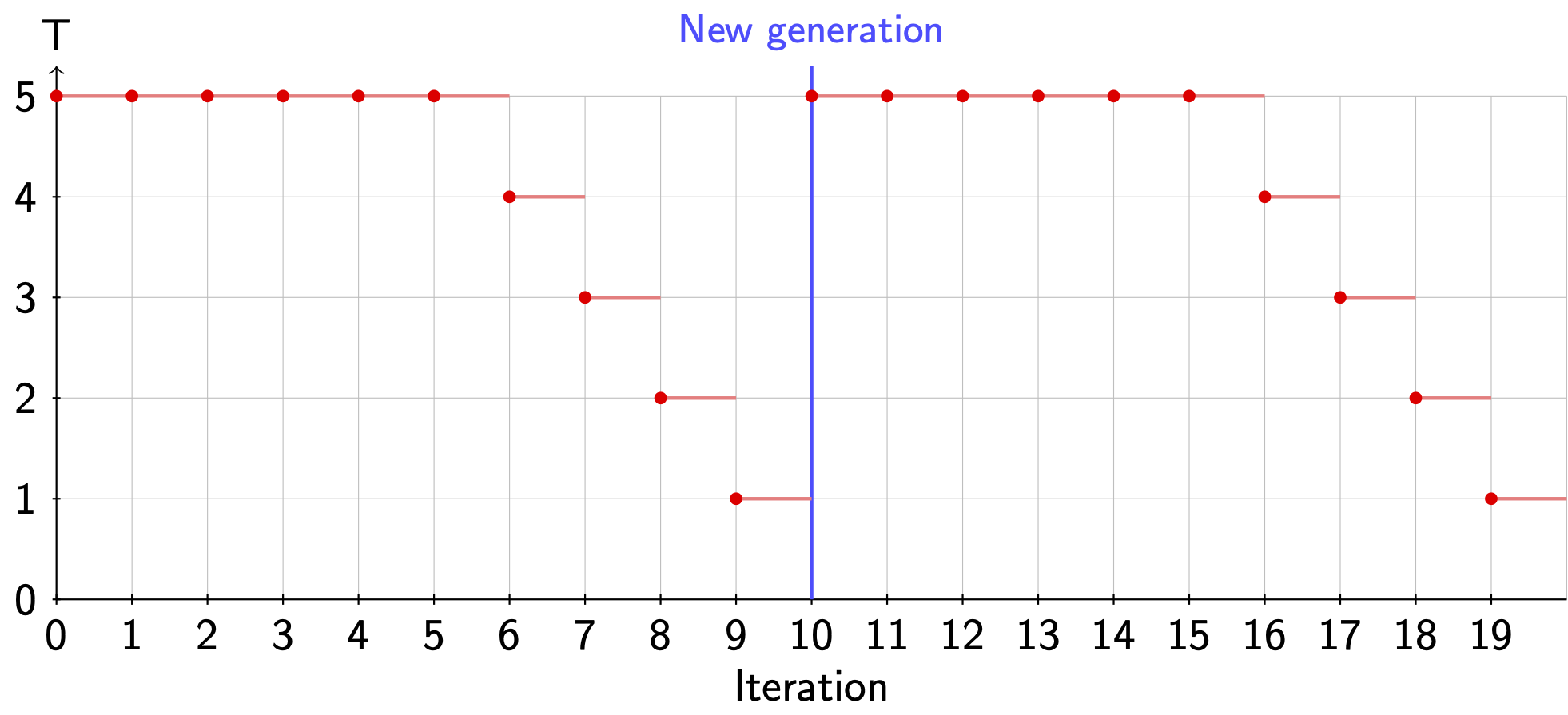
../_images/annealing_hybrid.png — Fig. 3.3 Annealing in the hybrid algorithm¶

However, when using the flag flag -anneal_globally, the starting temperature of the annealing will be decreased in steps at the beginning of each generation.